Read on TraderPlanet
Iced Coffee Anyone?
Just keeping up with the news, coffee should enter a lower priced environment, longer-term. In the short-run, technicals indicate an expectation of prices testing a threshold at 110 would not be unreasonable.
Coffee Production Forecast
Economists see much room for increased production out of Africa, which used to be the planet’s biggest crop exporter, producing 25 percent of the world’s coffee. After many years of state interference in, and regulation of agriculture, coffee production per acre is so low that it could fairly easily be increased by a factor of five. Simple changes have already increased output per tree by 50 percent in some areas. Incubator commodity firms are proving increases are practical. So, more supply means eventual lower prices.
Near-term Coffee Technical Indicators
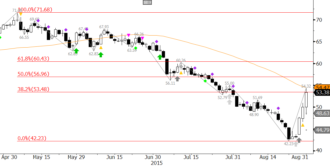
We’ve been bearish technically on coffee since our previous article that focused on the September contract, June 23 Will the Sun Shine on KC. We expected coffee to break down out of its correction, first to 123.2 and then to at least 117.50. 141 was resistance. KCU15 dropped to 123.65, rose to 139, coming within 2 cents of our level, then hit 117.5 exactly before meandering down to 113.05.
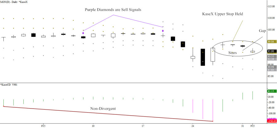
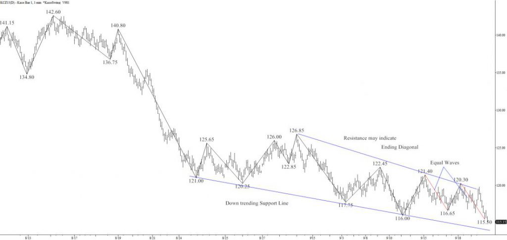
Given coffee’s back in the news, let’s look at the December contract. The chart patterns are unrelievedly negative on the daily chart and above. The intraday chart been bouncing along a downwardly sloping trend line. The market is attempting to skid to a halt, or at least a stall. The pattern intersects the y-axis at about 114.6. This is highly confluent, major support, as 114.6 is the smallest (0.62) extension for the wave down from 207.8, as well as, both extension targets and corrective projections for more recent waves. It’s also the endpoint of a rare ending diagonal triangle.
Coffee Outlook
I think 114.6 will break, even if there’s a bounce. The 122 – 125 area must be solidly overcome for a recovery to begin. On a slip below 114.6, I’d look for 110.6. One reason 114.6 will probably break is that the first of the two equal waves shown in red targets 112.7 as its 1.62 extension, showing no support at 114.6.
There might be a test of and small bounce after 112.7, which is “sandwiched” between 114.6 and 110.6 within the wave structure. So the three prices are connected making it more probable for the lower number to be met on a break through 114.6. Given that KCZ15 is making new contract lows, there’s not many numeric methods, aside from the waves to confirm the values discussed, though the daily warning line on Kase’s stops is 114.6.
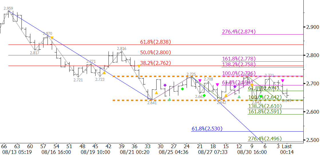
Unlike September, this contract has no support around 100.0. There’s big gap in the targets from 110.6 to 98.6. That means coffee wants to stay at least in the teens, and may move into a corrective phase into the 130s. So, I’d stay short, or day-trade short, but there might not be enough downside here for a longer lived position. Watch 110.6, and don’t crunch your ice.
Charts created using TradeStation. ©TradeStation Technologies, Inc. 2001-2015. All rights reserved. No investment or trading advice, recommendation or opinions are being given or intended.
Send questions for next week to askkase@kaseco.com, and click the link learn more about the KasePO, KaseCD, KEES, and the Kase DevStops.
 by
by 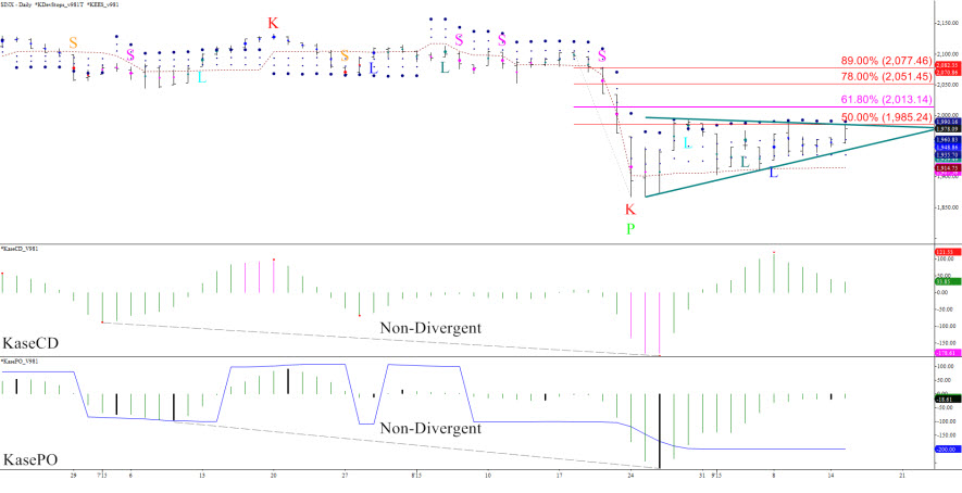 Charts created using TradeStation. ©TradeStation Technologies, Inc. 2001-2015. All rights reserved. No investment or trading advice, recommendation or opinions are being given or intended.
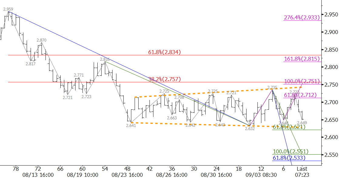

 By
By  Charts created using TradeStation. ©TradeStation Technologies, Inc. 2001-2015. All rights reserved. No investment or trading advice, recommendation or opinions are being given or intended.
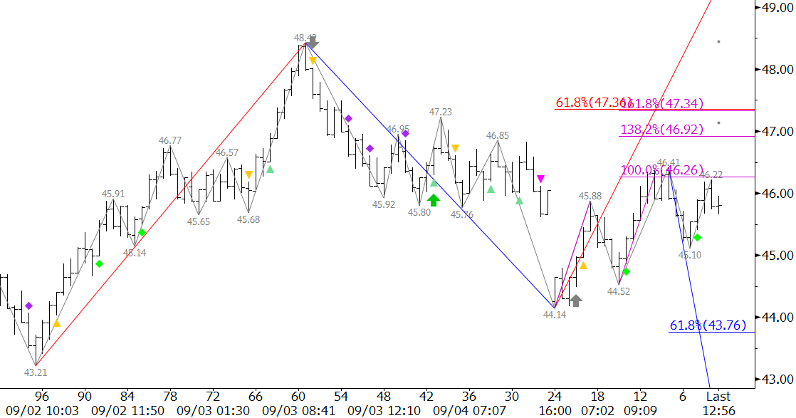
 By
By